Computational 2D Materials Database (C2DB)
If you are using data from this database in your research, please cite the following papers:
Article
Sten Haastrup, Mikkel Strange, Mohnish Pandey, Thorsten Deilmann, Per S. Schmidt, Nicki F. Hinsche, Morten N. Gjerding, Daniele Torelli, Peter M. Larsen, Anders C. Riis-Jensen, Jakob Gath, Karsten W. Jacobsen, Jens Jørgen Mortensen, Thomas Olsen, Kristian S. Thygesen
2D Materials 5, 042002 (2018)
Article
Recent Progress of the Computational 2D Materials Database (C2DB)
M. N. Gjerding, A. Taghizadeh, A. Rasmussen, S. Ali, F. Bertoldo, T. Deilmann, U. P. Holguin, N. R. Knøsgaard, M. Kruse, A. H. Larsen, S. Manti, T. G. Pedersen, T. Skovhus, M. K. Svendsen, J. J. Mortensen, T. Olsen, K. S. Thygesen
2D Materials 8, 044002 (2021)
The full dataset is provided upon request.
Brief description
The database contains structural, thermodynamic, elastic, electronic, magnetic, and optical properties of around 4000 two-dimensional (2D) materials distributed over more than 40 different crystal structures. The properties are calculated by density functional theory (DFT) and many-body perturbation theory (\(G_0W_0\) and the Bethe- Salpeter Equation for around 300 materials) as implemented in the GPAW electronic structure code. The workflow was constructed using the Atomic Simulation Recipes (ASR) and executed with the MyQueue task manager. The workflow script and a table with the numerical settings employed for the calculation of the different properties are provided below.
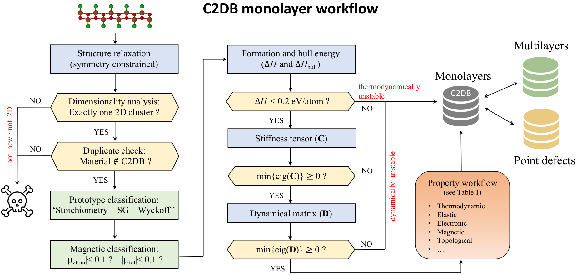
Overview of methods and parameters used
If a parameter is not specified at a given step, its value equals that of the last step where it was specified:
Workflow step(s) |
Parameters |
|---|---|
Structure and energetics(*) (1-4) |
vacuum = 15 Å; \(k\)-point density = 6.0/Å\(^{-1}\); Fermi smearing = 0.05 eV; PW cutoff = 800 eV; xc functional = PBE; maximum force = 0.01 eV/Å; maximum stress = 0.002 eV/Å\(^3\); phonon displacement = 0.01Å |
Elastic constants (5) |
\(k\)-point density = \(12.0/\mathrm{Å}^{-1}\); strain = \(\pm\)1% |
Magnetic anisotropy (6) |
\(k\)-point density = \(20.0/\mathrm{Å}^{-1}\); spin-orbit coupling = True |
PBE electronic properties (7-10 and 12) |
\(k\)-point density = \(12.0/\mathrm{Å}^{-1}\) (\(36.0/\mathrm{Å}^{-1}\) for DOS) |
Effective masses (11) |
\(k\)-point density = \(45.0/\mathrm{Å}^{-1}\); finite difference |
Deformation potential (13) |
\(k\)-point density = 12.0/Å\(^{-1}\); strain = \(\pm\)1% |
Plasma frequency (14) |
\(k\)-point density = 20.0/Å\(^{-1}\); tetrahedral interpolation |
HSE band structure (8-12) |
HSE06@PBE; \(k\)-point density = 12.0/Å\(^{-1}\) |
\(G_0W_0\) band structure (8, 9) |
\(G_0W_0\)@PBE; \(k\)-point density = \(5.0/\mathrm{Å}^{-1}\); PW cutoff = \(\infty\) (extrapolated from 170, 185 and 200 eV); full frequency integration; analytical treatment of \(W({q})\) for small \(q\); truncated Coulomb interaction |
RPA polarisability (15) |
RPA@PBE; \(k\)-point density = \(20.0/\mathrm{Å}^{-1}\); PW cutoff = 50 eV; truncated Coulomb interaction; tetrahedral interpolation |
BSE absorbance (16) |
BSE@PBE with \(G_0W_0\) scissors operator; \(k\)-point density = \(20.0/\mathrm{Å}^{-1}\); PW cutoff = 50 eV; truncated Coulomb interaction; at least 4 occupied and 4 empty bands |
(*) For the cases with convergence issues, we set a (k)-point density of 9.0 and a smearing of 0.02 eV.
Funding acknowledgements
The C2DB project has received funding from the Danish National Research Foundation’s Center for Nanostructured Graphene (CNG) and the European Research Council (ERC) under the European Union’s Horizon 2020 research and innovation program Grant No. 773122 (LIMA) and Grant agreement No. 951786 (NOMAD CoE).
Versions
Version |
rows |
comment |
2018-06-01 |
1888 |
Initial release |
2018-08-01 |
2391 |
Two new prototypes added |
2018-09-25 |
3084 |
New prototypes |
2018-12-10 |
3331 |
Some BSE spectra recalculated due to small bug affecting absorption strength of materials with large spin-orbit couplings |
2021-04-22 |
4049 |
Major update including several hundreds new monolayers from experimentally known crystals (from the ICSD/COD databases), new crystal prototype characterization scheme, improved properties (stiffness tensor, effective masses, optical absorbance), and new properties (exfoliation energies, Bader charges, spontaneous polarisations, Born charges, infrared polarisabilities, piezoelectric tensors, band topology invariants, exchange couplings, Raman- and second harmonic generation spectra). See Gjerding et al. for a full description. |
2021-06-24 |
4056 |
Updated MARE for effective masses. |
2022-09-08 |
15686 |
Added 11.630 materials from lattice decoration and a deep generative model (see arXiv:2206.12159). Corrected symmetry threshold used to define band structure path to be consistent with the threshold used to define the space group. |
2022-11-30 |
15733 |
Shift currents for selected materials. Improved deformation potentials. |
2024-05-01 |
16789 |
New webpages. Restructuring of the search page (removed HIGH, MEDIUM, LOW characterization of thermodynamic stability). Added various properties for the 3.330 most stable of the 11.630 structures that were added in version 2022-09-08. Added ca. 100 self-intercalated bilayers. Spontaneous polarisations for 63 ferroelectrics. Symmetry classification according to layer groups in addition to space groups of the AA-stacked bulk. |
Key-value pairs
See available keys here.
Using the data
Here is an example using the c2db.db ASE-DB file:
import matplotlib.pyplot as plt
from ase.db import connect

db = connect('c2db.db')
rows = db.select('gap_gw')

gw = []
hse = []
pbe = []
for row in rows:
    gw.append(row.gap_gw)
    hse.append(row.gap_hse)
    pbe.append(row.gap)

fig = plt.figure()
ax = fig.add_subplot(1, 1, 1)
ax.plot(pbe, hse, 'o', label='HSE06')
ax.plot(pbe, gw, 'x', label='GW')
x = [0, max(pbe)]
ax.plot(x, x, label='PBE')
ax.set_xlabel('PBE-gap [eV]')
ax.set_ylabel('gap [eV]')
ax.legend()
plt.savefig('gaps.png')
Alternatively, one can unpack the c2db.tar.gz file with
tar -xf c2db.tar.gz and extract the gaps like this:
from pathlib import Path
import json

gw = []
hse = []
pbe = []
for path in Path().glob('materials/A*/*/*'):
    data = json.loads((path / 'data.json').read_text())
    if 'gap_gw' in data:
        gw.append(data['gap_gw'])
        hse.append(data['gap_hse'])
        pbe.append(data['gap'])